In this post, common machine learning techniques, such as feature engineering, data transformation, Cross validation, and hyperparameter tuning are applied to a several regression-based and tree-based classifiers. For this comparative analysis the Covertype dataset from UCI machine learning repository is used to predict the type of forest coverage from one of the 7 categories. This is a single-label multi-class classification with equal weight classes.
For this work we selected the following multi-class classifiers:
- Logistic Regression
- Ridge Regression
- Random Forest
- Gradient Boosting
- XGBoost
- Dataset information: Researchers at the Department of Forest Sciences at Colorado State University collected over half a million measurements from tree observations from four areas of the Roosevelt National Forest in Colorado. All observations are cartographic variables (no remote sensing) from 30-meter x 30-meter sections of forest. The resulting dataset includes information on tree type, shadow coverage, distance to nearby landmarks (roads etcetera), soil type, and local topography. This dataset was obtained from UCI machine learning repository. It contains 15120 observations and 56 columns in total. This data includes 7 categories of different cover types, which will be used as the target label for prediction, 10 continuous variables, and 2 categorical variables, Wilderness areas and soil types. The categorical variables are encoded with one hot encoder.
Bache, K. & Lichman, M. (2013). UCI Machine Learning Repository. Irvine, CA: University of California, School of Information and Computer Science
Loading dataset
# Import data
import pandas as pd
import numpy as np

data = pd.read_csv('https://github.com/skhabiri/PredictiveModeling-CoverType-u2build/blob/master/data/train.csv?raw=true')
print(data.shape)
data.head()
(15120, 56)
| Id | Elevation | Aspect | Slope | Horizontal_Distance_To_Hydrology | Vertical_Distance_To_Hydrology | Horizontal_Distance_To_Roadways | Hillshade_9am | Hillshade_Noon | Hillshade_3pm | Horizontal_Distance_To_Fire_Points | Wilderness_Area1 | Wilderness_Area2 | Wilderness_Area3 | Wilderness_Area4 | Soil_Type1 | Soil_Type2 | Soil_Type3 | Soil_Type4 | Soil_Type5 | Soil_Type6 | Soil_Type7 | Soil_Type8 | Soil_Type9 | Soil_Type10 | Soil_Type11 | Soil_Type12 | Soil_Type13 | Soil_Type14 | Soil_Type15 | Soil_Type16 | Soil_Type17 | Soil_Type18 | Soil_Type19 | Soil_Type20 | Soil_Type21 | Soil_Type22 | Soil_Type23 | Soil_Type24 | Soil_Type25 | Soil_Type26 | Soil_Type27 | Soil_Type28 | Soil_Type29 | Soil_Type30 | Soil_Type31 | Soil_Type32 | Soil_Type33 | Soil_Type34 | Soil_Type35 | Soil_Type36 | Soil_Type37 | Soil_Type38 | Soil_Type39 | Soil_Type40 | Cover_Type | |
|---|---|---|---|---|---|---|---|---|---|---|---|---|---|---|---|---|---|---|---|---|---|---|---|---|---|---|---|---|---|---|---|---|---|---|---|---|---|---|---|---|---|---|---|---|---|---|---|---|---|---|---|---|---|---|---|---|
| 0 | 1 | 2596 | 51 | 3 | 258 | 0 | 510 | 221 | 232 | 148 | 6279 | 1 | 0 | 0 | 0 | 0 | 0 | 0 | 0 | 0 | 0 | 0 | 0 | 0 | 0 | 0 | 0 | 0 | 0 | 0 | 0 | 0 | 0 | 0 | 0 | 0 | 0 | 0 | 0 | 0 | 0 | 0 | 0 | 1 | 0 | 0 | 0 | 0 | 0 | 0 | 0 | 0 | 0 | 0 | 0 | 5 |
| 1 | 2 | 2590 | 56 | 2 | 212 | -6 | 390 | 220 | 235 | 151 | 6225 | 1 | 0 | 0 | 0 | 0 | 0 | 0 | 0 | 0 | 0 | 0 | 0 | 0 | 0 | 0 | 0 | 0 | 0 | 0 | 0 | 0 | 0 | 0 | 0 | 0 | 0 | 0 | 0 | 0 | 0 | 0 | 0 | 1 | 0 | 0 | 0 | 0 | 0 | 0 | 0 | 0 | 0 | 0 | 0 | 5 |
| 2 | 3 | 2804 | 139 | 9 | 268 | 65 | 3180 | 234 | 238 | 135 | 6121 | 1 | 0 | 0 | 0 | 0 | 0 | 0 | 0 | 0 | 0 | 0 | 0 | 0 | 0 | 0 | 1 | 0 | 0 | 0 | 0 | 0 | 0 | 0 | 0 | 0 | 0 | 0 | 0 | 0 | 0 | 0 | 0 | 0 | 0 | 0 | 0 | 0 | 0 | 0 | 0 | 0 | 0 | 0 | 0 | 2 |
| 3 | 4 | 2785 | 155 | 18 | 242 | 118 | 3090 | 238 | 238 | 122 | 6211 | 1 | 0 | 0 | 0 | 0 | 0 | 0 | 0 | 0 | 0 | 0 | 0 | 0 | 0 | 0 | 0 | 0 | 0 | 0 | 0 | 0 | 0 | 0 | 0 | 0 | 0 | 0 | 0 | 0 | 0 | 0 | 0 | 0 | 1 | 0 | 0 | 0 | 0 | 0 | 0 | 0 | 0 | 0 | 0 | 2 |
| 4 | 5 | 2595 | 45 | 2 | 153 | -1 | 391 | 220 | 234 | 150 | 6172 | 1 | 0 | 0 | 0 | 0 | 0 | 0 | 0 | 0 | 0 | 0 | 0 | 0 | 0 | 0 | 0 | 0 | 0 | 0 | 0 | 0 | 0 | 0 | 0 | 0 | 0 | 0 | 0 | 0 | 0 | 0 | 0 | 1 | 0 | 0 | 0 | 0 | 0 | 0 | 0 | 0 | 0 | 0 | 0 | 5 |
All the columns have int dtype. * The dataset has 15120 rows and 56 columns. This is a multiclass classification with “Cover_Type” as the target label. Wilderness_Area and Soil_Type columns have been encoded with One Hot Encoder. For better visualization, we will convert all the Soil_Types and Wilderness_Areas columns into two categorical features “Soil_Type” and “Wilderness_Area”.
data1 = data.copy()
# Encode Soil_Types and Wilderness_Area features into two new features
ohe_bool = []
enc_cols = ["Wilderness_Area", "Soil_Type"]
for idx, val in enumerate(enc_cols):
  val_df = data.filter(regex=val, axis=1)
  print(f"{idx} {val} is ohe? {((val_df.sum(axis=1)) == 1).all()}")
  data1[val] = val_df.dot(val_df.columns)
  # Convert the constructed columns into int
  data1[val] = data1[val].astype('str').str.findall(r"(\d+)").str[-1].astype('int')
  data1 = data1.drop(val_df.columns, axis=1)

# Reorder the columns
data1 = data1.iloc[:,data1.columns!="Cover_Type"].merge(data1["Cover_Type"], left_index=True, right_index=True)
data1.head(), data1.shape
(15120, 14)
| Id | Elevation | Aspect | Slope | Horizontal_Distance_To_Hydrology | Vertical_Distance_To_Hydrology | Horizontal_Distance_To_Roadways | Hillshade_9am | Hillshade_Noon | Hillshade_3pm | Horizontal_Distance_To_Fire_Points | Wilderness_Area | Soil_Type | Cover_Type | |
|---|---|---|---|---|---|---|---|---|---|---|---|---|---|---|
| 0 | 1 | 2596 | 51 | 3 | 258 | 0 | 510 | 221 | 232 | 148 | 6279 | 1 | 29 | 5 |
| 1 | 2 | 2590 | 56 | 2 | 212 | -6 | 390 | 220 | 235 | 151 | 6225 | 1 | 29 | 5 |
| 2 | 3 | 2804 | 139 | 9 | 268 | 65 | 3180 | 234 | 238 | 135 | 6121 | 1 | 12 | 2 |
| 3 | 4 | 2785 | 155 | 18 | 242 | 118 | 3090 | 238 | 238 | 122 | 6211 | 1 | 30 | 2 |
| 4 | 5 | 2595 | 45 | 2 | 153 | -1 | 391 | 220 | 234 | 150 | 6172 | 1 | 29 | 5 |
data1.describe()
| Id | Elevation | Aspect | Slope | Horizontal_Distance_To_Hydrology | Vertical_Distance_To_Hydrology | Horizontal_Distance_To_Roadways | Hillshade_9am | Hillshade_Noon | Hillshade_3pm | Horizontal_Distance_To_Fire_Points | Wilderness_Area | Soil_Type | Cover_Type | |
|---|---|---|---|---|---|---|---|---|---|---|---|---|---|---|
| count | 15120.00000 | 15120.000000 | 15120.000000 | 15120.000000 | 15120.000000 | 15120.000000 | 15120.000000 | 15120.000000 | 15120.000000 | 15120.000000 | 15120.000000 | 15120.000000 | 15120.000000 | 15120.000000 |
| mean | 7560.50000 | 2749.322553 | 156.676653 | 16.501587 | 227.195701 | 51.076521 | 1714.023214 | 212.704299 | 218.965608 | 135.091997 | 1511.147288 | 2.800397 | 19.171362 | 4.000000 |
| std | 4364.91237 | 417.678187 | 110.085801 | 8.453927 | 210.075296 | 61.239406 | 1325.066358 | 30.561287 | 22.801966 | 45.895189 | 1099.936493 | 1.119832 | 12.626960 | 2.000066 |
| min | 1.00000 | 1863.000000 | 0.000000 | 0.000000 | 0.000000 | -146.000000 | 0.000000 | 0.000000 | 99.000000 | 0.000000 | 0.000000 | 1.000000 | 1.000000 | 1.000000 |
| 25% | 3780.75000 | 2376.000000 | 65.000000 | 10.000000 | 67.000000 | 5.000000 | 764.000000 | 196.000000 | 207.000000 | 106.000000 | 730.000000 | 2.000000 | 10.000000 | 2.000000 |
| 50% | 7560.50000 | 2752.000000 | 126.000000 | 15.000000 | 180.000000 | 32.000000 | 1316.000000 | 220.000000 | 223.000000 | 138.000000 | 1256.000000 | 3.000000 | 17.000000 | 4.000000 |
| 75% | 11340.25000 | 3104.000000 | 261.000000 | 22.000000 | 330.000000 | 79.000000 | 2270.000000 | 235.000000 | 235.000000 | 167.000000 | 1988.250000 | 4.000000 | 30.000000 | 6.000000 |
| max | 15120.00000 | 3849.000000 | 360.000000 | 52.000000 | 1343.000000 | 554.000000 | 6890.000000 | 254.000000 | 254.000000 | 248.000000 | 6993.000000 | 4.000000 | 40.000000 | 7.000000 |
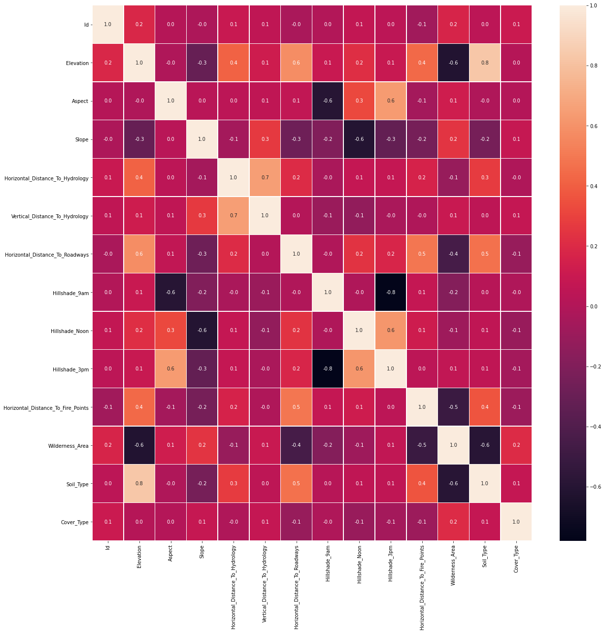
Next we plot the Heatmap of correlation matrix. It shows Elevation and Soil_Type are highly correlated, and Hillshade_3pm is reversely correlated with Hillshade_9am.
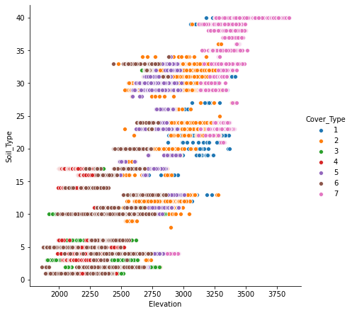
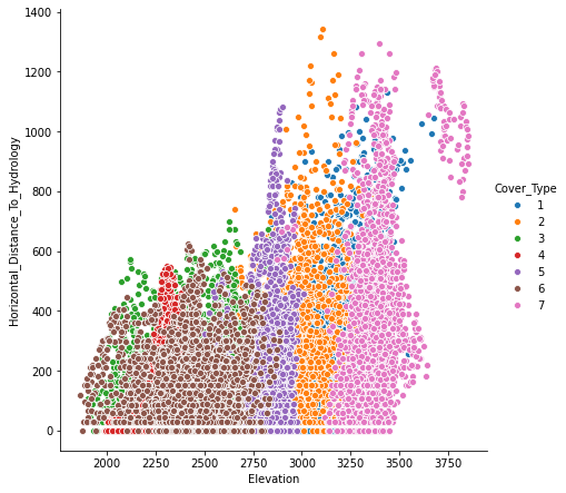
Looking at scatter plot of different features, it seems “Elevation” is an important parameter in separating different classes of target label.
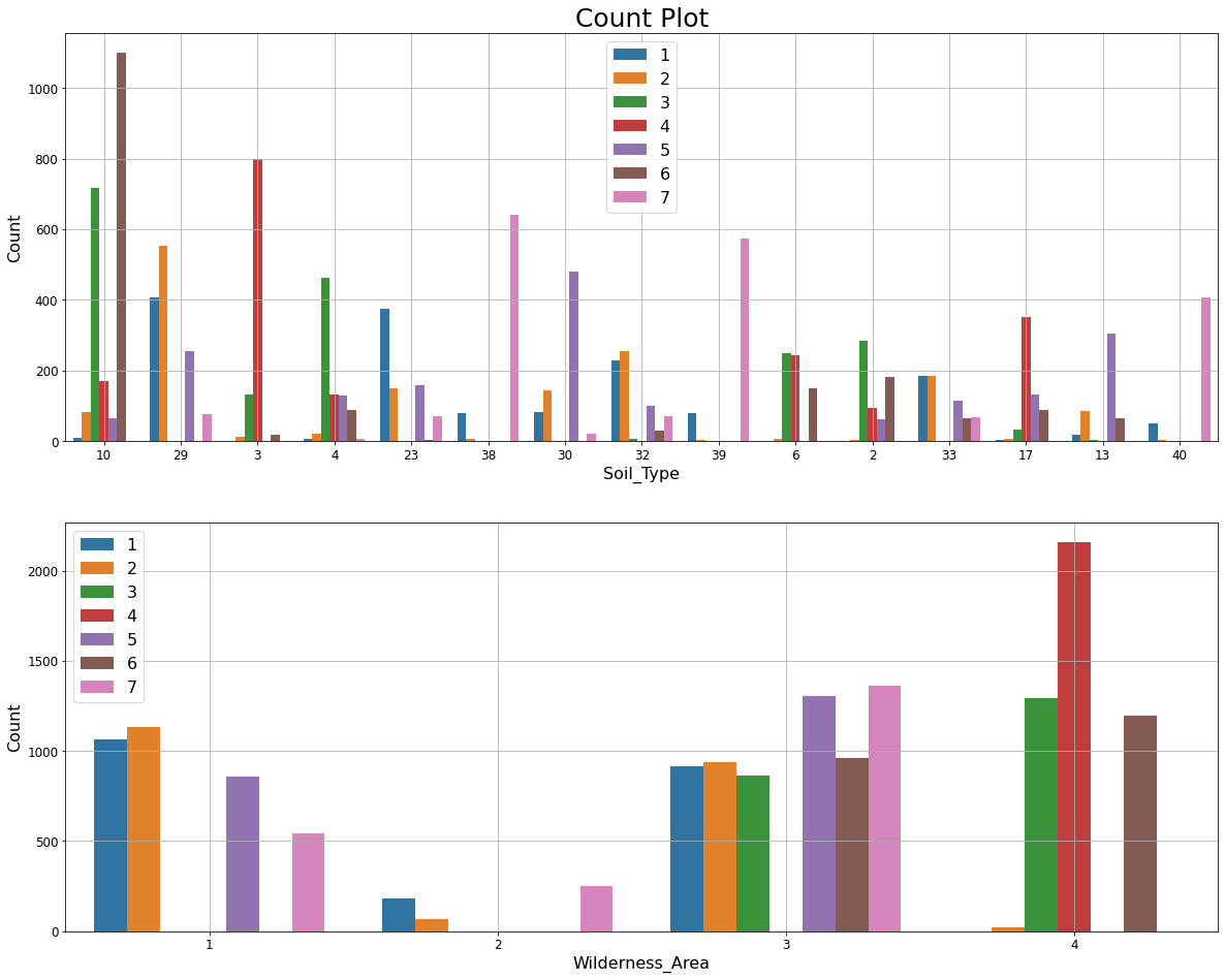
We make the following observations from the Count plots below.
- Soil_Type10 shows a significant class distinction for Cover_Type=6.
- Similarly Wilderness_Area4 and Cover_Type=4 are strongly associated.
List of unique values in the feature shows Soil_Type15 and Soil_Type7 are constant. Additionally, Id column is a unique identifier for each observation. We’ll drop those three columns as they do not carry any information to identify the target label.
There are also skewness in some features. “Horizontal_Distance_To_Hydrology” is an example of that.

Train-Test Split
After removing “Id” and constant columns, data is split into train and validation set.
from sklearn.model_selection import train_test_split
# Split train into train & val
train, val = train_test_split(data, train_size=0.80, test_size=0.20, stratify=data["Cover_Type"], random_state=42)
# Separate class label and data
y_train = train["Cover_Type"]
X_train = train.drop("Cover_Type", axis=1)
y_val = val["Cover_Type"]
X_val = val.drop("Cover_Type", axis=1)
print(f'train: {train.shape}, val: {val.shape}')
train: (12096, 56), val: (3024, 56)
Baseline model
Normalized value counts of the target label shows an equal weight distribution for all classes, with baseline prediction of 14.3%.
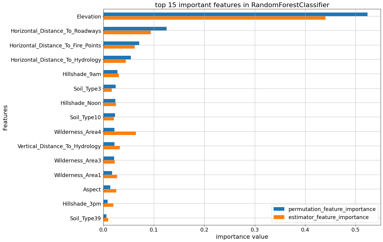
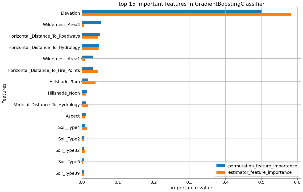
Pipeline Estimators, Feature_importances and permutation_importance
We are going to look at five different classifiers to compare their performance. For the regression classifiers we will standardize the data before fitting.
- LogesticRegression
- RidgeClassifier
- RandomForestClassifier
- GradientBoostingClassifier
- XGBCLassifier
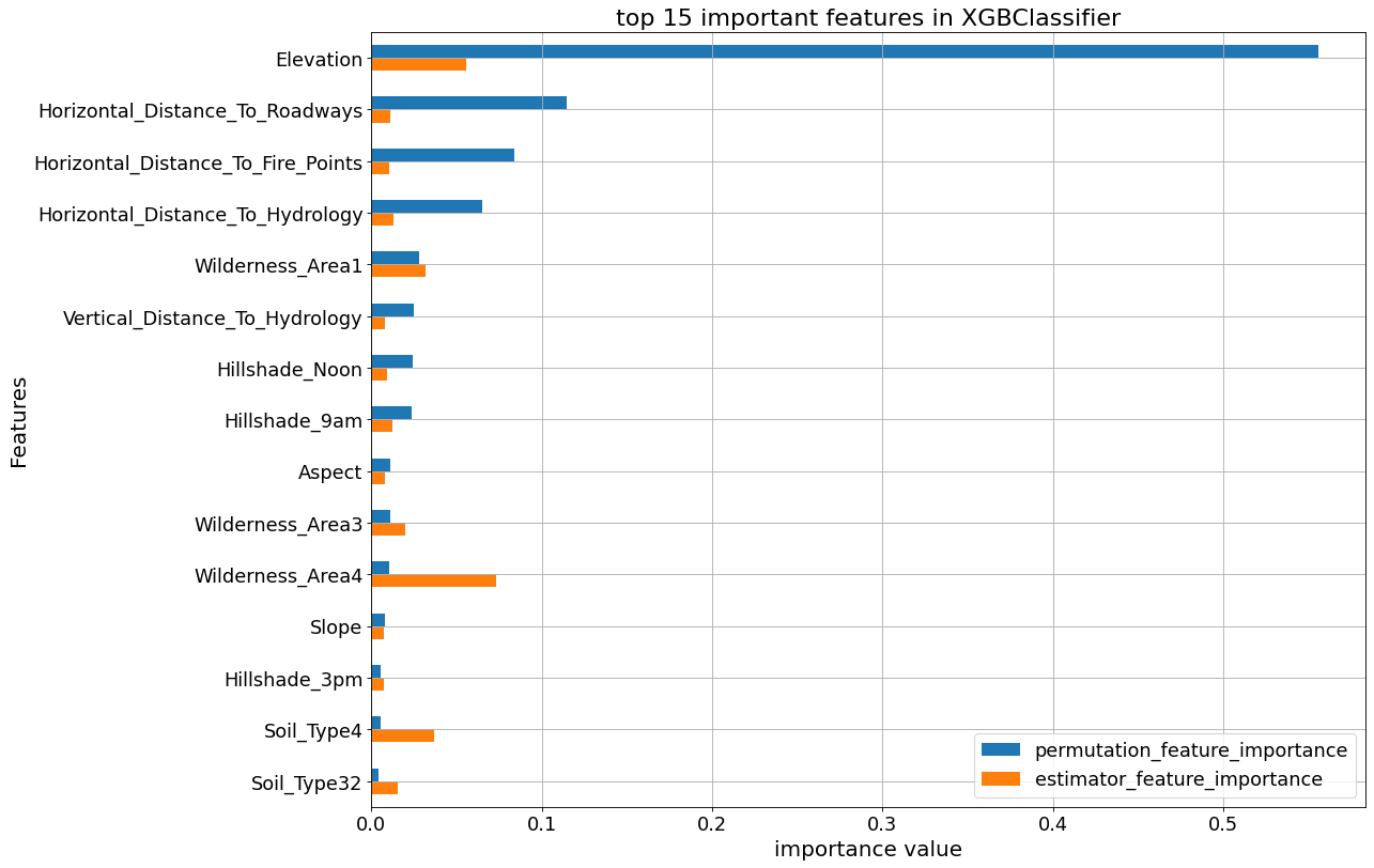
The following plots show the feature_importances and permutation importances of the tree-base classifiers. “Elevation” is given a higher importance weight compared to other features, as we saw earlier. Without the help of permutation, XGBClassifier does not seem to detect the importance of “Elevation” feature.
Avoid Overfitting By Early Stop feature in XGBoost Classifier
XGBClassifier tends to overfit and its growth parameters need to be controlled. To demonstrate that, an early stop fitting with 50 rounds is run below. We notice at some point in fitting process the validation error stops decreasing steady.
# XGBoost early stop fit
xform = make_pipeline(
    FunctionTransformer(wrangle, validate=False),
    # ce.OrdinalEncoder(),
)

xform.set_params(functiontransformer__kw_args = kwargs_dict)

X_train_xform = xform.fit_transform(X_train)
X_val_xform = xform.transform(X_val)

clf = XGBClassifier(
    n_estimators = 1000,
    max_depth=8,
    learning_rate=0.5,
    num_parallel_tree = 10,
    n_jobs=-1
)

#eval_set
eval_set = [(X_train_xform, y_train), (X_val_xform, y_val)]

clf.fit(X_train_xform, y_train,
          eval_set=eval_set,
          eval_metric=['merror', 'mlogloss'],
          early_stopping_rounds=50,
          verbose=False) # Stop if the score hasn't improved in 50 rounds

print('Training Accuracy:', clf.score(X_train_xform, y_train))
print('Validation Accuracy:', clf.score(X_val_xform, y_val))
Training Accuracy: 0.9987599206349206 Validation Accuracy: 0.8528439153439153
XGBoost trains upto 0.999 and yields 0.85 validation accuracy. The following graph shows how validation error remains constant while training error reduces.

Cross Validation Curve
The training set is split into kfolds and the model is cross validated based on a classifier parameter.
kfold=4
for k, estimator in enumerate(tree_list):
  print(f"********** {est_dict[estimator][0].__class__.__name__} **********")
  classifier_name = clf_name(estimator, est_dict)
  # estimator.set_params(functiontransformer__kw_args = kwargs_dict)
  # print(est_dict[estimator][1])

  param_distributions = {classifier_name.lower()+'__'+ est_dict[estimator][1][j]: est_dict[estimator][2][j] for j in range(len(est_dict[estimator][1]))}

  for i in range(len(est_dict[estimator][1])):
    param_name=classifier_name.lower()+'__'+ est_dict[estimator][1][i]
    param_range = est_dict[estimator][2][i]
    estimator.set_params(functiontransformer__kw_args = kwargs_dict)

    train_scores, val_scores = validation_curve(estimator, X_train, y_train,
    # param_name='functiontransformer__kw_args',
    param_name=param_name,
    param_range=param_range,
    scoring='accuracy', cv=kfold, n_jobs=-1, verbose=0
    )

    print(f'**** {param_name} ****\n')
    print("val scores mean:\n", np.mean(val_scores, axis=1))

    # Averaging CV scores
    fig, ax = plt.subplots(figsize=(12,8))

    ax.plot(param_range, np.mean(train_scores, axis=1), color='blue', label='mean training accuracy')
    ax.plot(param_range, np.mean(val_scores, axis=1), color='red', label='mean validation accuracy')
    ax.set_title(f'Cross Validation with {kfold:d} folds', fontsize=20)
    ax.set_xlabel(param_name, fontsize=18)
    ax.set_ylabel('model score: Accuracy', fontsize=18)
    ax.legend(fontsize=12)
    ax.tick_params(axis='both', labelsize=16)
    ax.grid(which='both')
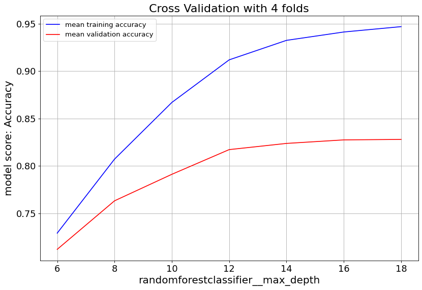
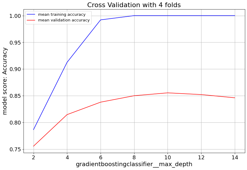
Gradient Boost classifier family quickly overfit at max_depth>6. So it’s important to keep the tree depth shallow.
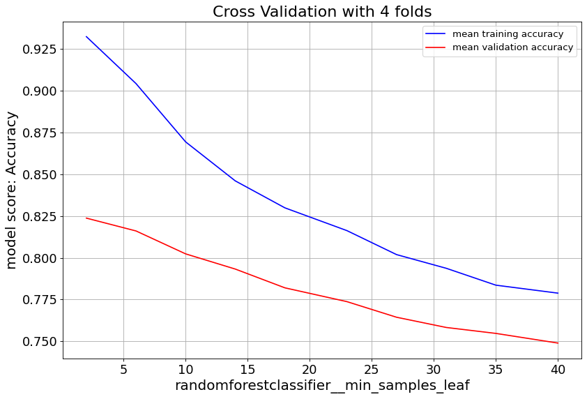
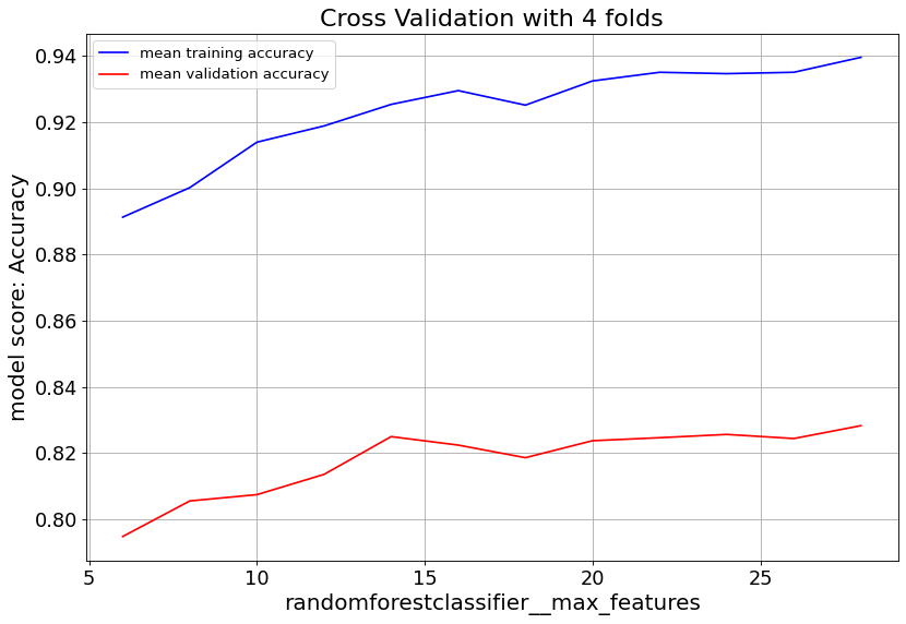
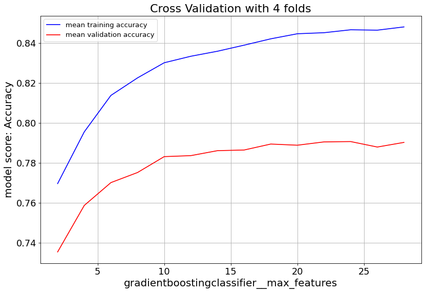
max_feat parameter shows validation score saturates at numbers above 20, and starts to overfit. Lowering min_samples_leaf improves validation score. Hence we consider small numbers.
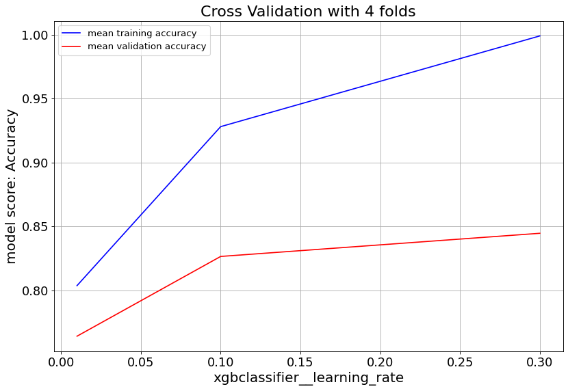
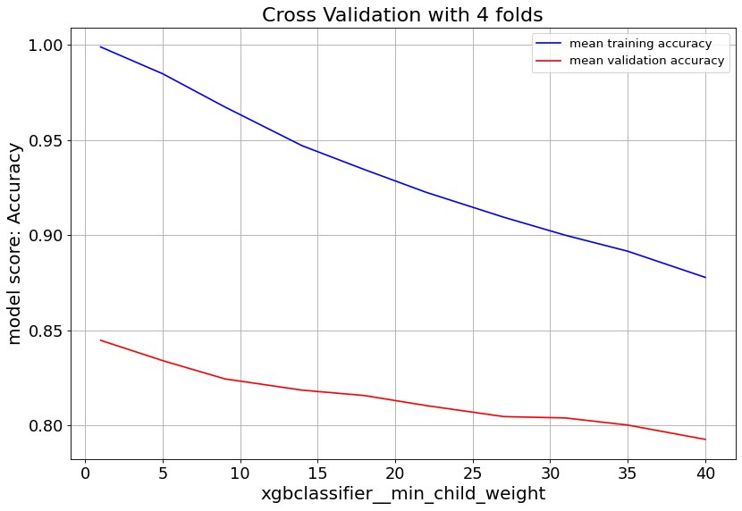
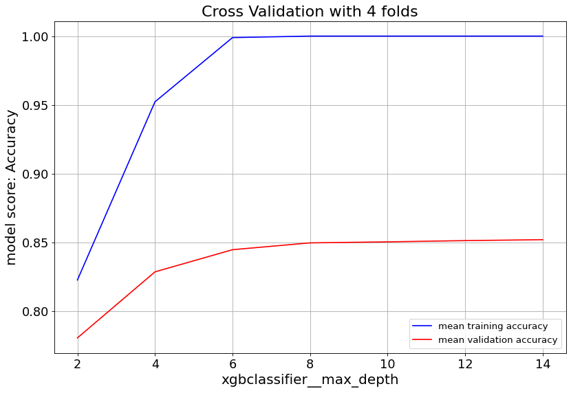
For XGBoost we can slow down the overfitting issue with min_child_weight and learningrate parameters.
Hyper Parameter Tunning
The parameters of all five estimators are optimized by RandomizedSearchCV.
kfold=4
n_iter = 10
best_ests = [np.NaN]*len(est)
best_scores = [np.NaN]*len(est)
best_params = [np.NaN]*len(est)

for i, estimator in enumerate(est):
  print(f"\n********** {est_dict[estimator][0].__class__.__name__} **********")
  estimator.set_params(functiontransformer__kw_args = kwargs_dict)

  classifier_name = clf_name(estimator=estimator, est_dict=est_dict)
  print(est_dict[estimator][1])

  param_distributions = {classifier_name.lower()+'__'+ est_dict[estimator][1][j]:
                         est_dict[estimator][2][j] for j in range(len(est_dict[estimator][1]))}

  rscv = RandomizedSearchCV(estimator, param_distributions=param_distributions,
    n_iter=n_iter, cv=kfold, scoring='accuracy', verbose=1, return_train_score=True,
    n_jobs=-1)

  rscv.fit(X_train, y_train)
  best_ests[i] = rscv.best_estimator_
  best_scores[i] = rscv.best_score_
  best_params[i] = rscv.best_params_

best_ypreds = [best_est.predict(X_val) for best_est in best_ests]
best_testscores = [accuracy_score(y_val, best_ypred) for best_ypred in best_ypreds]
print('Test accuracy\n', best_testscores)
print('best cross validation accuracy\n', best_scores)
Test accuracy [0.6911375661375662, 0.6326058201058201, 0.7754629629629629, 0.8700396825396826, 0.8498677248677249] best cross validation accuracy [0.7080026455026454, 0.6332671957671958, 0.7709986772486773, 0.8645833333333334, 0.8445767195767195]
The accuracy scores above corresponds to LogisticRegression, RidgeClassifier RandomForestClassifier, GradientBoostingClassifier, XGBClassifier accordingly. In this work, GradientBoostingClassifier with 87% accuracy on the test data shows the best performance among the five.
Conclusion
This post evaluates and compares the performance of five multi-class classifiers to predict the “Cover-Type” label of Covertype dataset. The dataset has 54 features, and one target label with 7 different classes. Target label classes are distributed evenly with baseline prediction of 14%. We splitted the total 15120 obeservations into train and test subsets. By applying commonly used classification methods such as feature selection, data scaling, cross validation, and hyperparameter optimization, we were able to achive accuracy scores ranging from 63% to 86% on test data subset. The score metrics of a typical fit of those classifiers has been deployed onto heroku.